This is an assignment from CMU 16720-A. In this assignment, I’m going to use Bag of Words to implement a scene classifier. I’m given a subset of the SUN Image database which consists of eight scene categories. Based on this dataset, I will build a visual words dictionary first, and then use those visual words to translate all images in that dataset. Next, I’ll get the histograms of the word number of every image. Then, I’ll map those histograms to a higher dimension space and use that space to do the classification.

Build Visual Words Dictionary

First, we are given four groups of filters generated by createFilterBank function. The first groups are the Gaussian filters, which have five different scales. The second group is the Laplacian filters. The third and fourth group are the derivatives of the first group with respect to the x-direction and y-direction.

If we apply those filters to the image, we can see something like below.

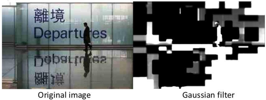
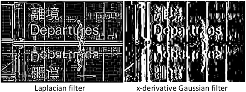
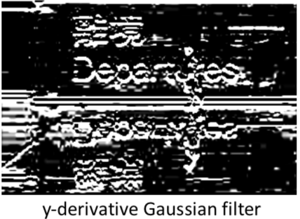
We can see that the Gaussian filter smooths the difference between pixel neighbors. The Laplacian filter extracts the edges. The x and y derivate Gaussian filters extract the vertical edges and horizontal edges respectively.

Because we have 20 filters, we will generate 20 new images for each image. After generating those new images, we are going to collect features from them. To collect features, we first determine which pixel location we are going to use, and then we collect pixel values from that 20 new images on the same location. For example, if we want to get the feature on (5,33), we will collect the pixel values on (5,33) from that 20 images. As a result, for one feature, the dimension will be 20×1.

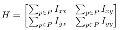
How do we decide the feature locations? The first one is random pixels locations. We are given the number of features () we need, and then we randomly generate coordinates. The next one is Harris corner detection algorithm. Here, we implement this algorithm by using below covariance matrix.

Then, we compute the R and select the \alpha biggest points.

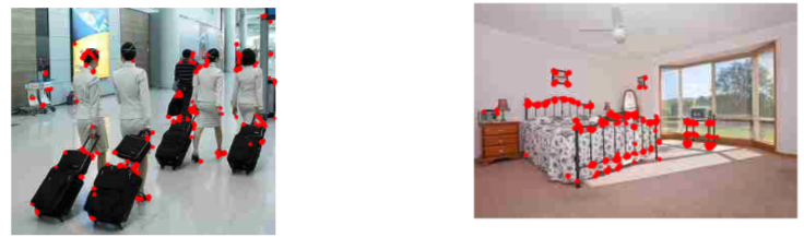
Below is the demo of Harris corner.

Once we get all the features from images, we can start building our dictionary. Here, the is 50, so we extract 50 features from each image. Since we have 1331 images for those 8 categories, we will have 1331*50 = 66550 features. Now, we use kmeans algorithm to cluster these 66550 points into 100 groups. So, right now we have 100 words in our visual words dictionary.

Bag of Words

In this part, we first translate every pixel of one image by using our 100 visual words. Then, we use the number of each word (histogram) in an image to do the classification.

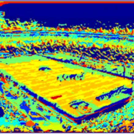
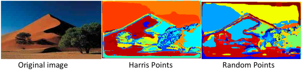
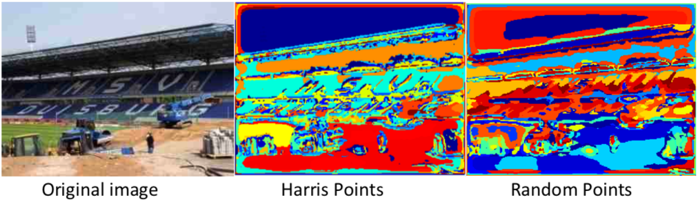
To translate, we need to go through previous getting features process again. However, instead of getting points, we get features from all of the points. Then, we use pdist2 to measure the Euclidean distance between the point A and our 100 words. We’ll say the point A is word X if the distance between feature A and X is the smallest. Below are the visualization results of the translation.

Now, for each image, we are going to compute the histogram of the word number from those 100 words. For example, for image1 we might have 259 word 1, 324 word 2, …, and so on. Since we only have 100 words, we can treat this histogram as a 100×1 vector. After we compute all the histograms of 1331 images, we now have 1331 100×1 vectors with labels.

Finally, for each test image, we find the nearest neighbor in the 100-degree space and look up its label and say “oh! they are the same category”. Now, we already built a scene classifier for images.

The accuracy of this scene classifier is around 50%, which is better than a random guess, but still not very good. One thing to be noticed is that the accuracy difference between random points selection and Harris corner algorithm is not very big. I think this is because when using Harris corner algorithm, our features are mostly from corners in the images. This will decrease the diversity of our features and thus the dictionary we built is more specific for corners. However, when we do the Bag of Words, we don’t just look at the corners, we want to translate all pixels in the images. This might make the translation less accurate.

Another thing to be noticed is that if we use chi2 for measuring distance when doing Bag of Words, the result will be better. I think this is because chi2 takes the word frequency into account. The more the word appears in these two images, the less important this difference should be because this word might be a common word and we can’t use its difference to tell anything. This is just like if A article has 75 “the”, and B article has “56” the, we can’t tell if they are similar or not. But if they both have more than 100 times “baseball”, we might guess they are in the same category.

Extra credit

Instead of the nearest neighbors, I also try to use SVM. The accuracy is slightly better than before. I try to use Inverse Document Frequency when computing the histogram, and the result is also only slightly better.