This is an assignment in CMU 16720-A. In this assignment, we implemented some basic image processing algorithms and use them to build a Hough Transform based line detector. We used Matlab to implement all of these functions. In the following sections, I will follow the structure of the assignment, but I will not disclose my code.

Convolution

Given an image and a filter h, we need to implement a function which performs the convolution operation with that filer h on the image. Because the definition of convolution is to reversely do the bitwise product, I first use im2col to transform the image and filter matrix into a column, use flipud to reverse the filter column, and then just dot product filter column and image column. Finally, we need to reshape the image column back to a new image.

Edge Detection

In this section, we are given an input image, and we want to return the x-direction gradient (Ix), y-direction gradient (Iy), the orientation of the image gradients (Io), and the magnitude of the image gradients (Im). Why do we want to get all those gradients? This is because the image pixel values change drastically on edges. To generate those gradients, we first use a Gaussian smoothing kernel to convolve the whole image, which reduces noises in this image. Then, we simply convolve our image with two Sobel filter (x and y-direction) respectively and get the Ix and Iy. The Io would be

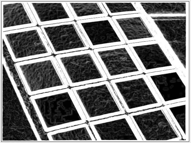
Typically, we want our edge to be a single line. However, after using Sobel filter, the edge (by looking at the magnitude region) will be very thick just like below.

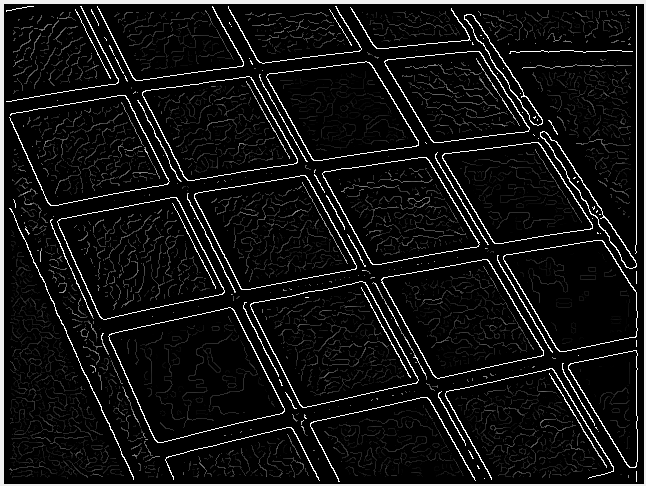
In order to fix this problem, we implement the non-maximal suppression. In the non-maximal suppression, for each pixel, we look at the two neighbors pixels along the gradient direction (Io) and if either of those pixels has a larger gradient magnitude, then we set the gradient magnitude of that pixel to zero. Here, we only consider 4 cases in the non-maximal suppression, which are 0°, 45°, 90°, and 135°. We map the gradient direction to the closest of the 4 cases. For example, 20° would map to 0°. After using the non-maximal suppression, the result becomes:

Now, we have already found a way to retrieve the edge pixels. However, we still can’t get the representation of edges. What we have now are only a bunch of pixels which have a non-zero value. We still want to find a representation, such as a slope and a y-intercept (y=ax+b), so that we can know exactly where those edges are. To do so, we will need Hough Transform.

Finding Lines

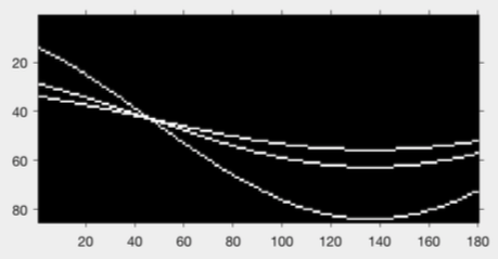
In the Hough Transform, we map a line from y=ax+b into . By using this transform, we can convert a point in an x-y plane into a curve in the Hough plane. Likewise, we can convert a point in Hough plane back to a line in the x-y plane. Knowing this property, we can now map the disjoint edge points we have before to the Hough plane. After this mapping, we will get many curves. The point with most intersections in Hough plane can then map back to the x-y plane as a line, which is the edge! If there are three dots in the x-y plane, the Hough plane will look like:

To implement Hough Transform, we just preallocate a , where is from -90° to 90° and is from 0 to (max ). Whenever we meet a point in the x-y plane, we add one to the cell in the curve on Hough plane. It is just like a voting mechanism. After we finish voting, we do a non-maximal suppression on Hough plane again. Then, we select the first N points in Hough plane so that we can map them back to a line in the x-y plane. Then, we can get something like below.

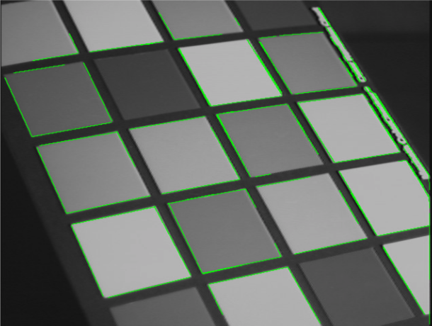
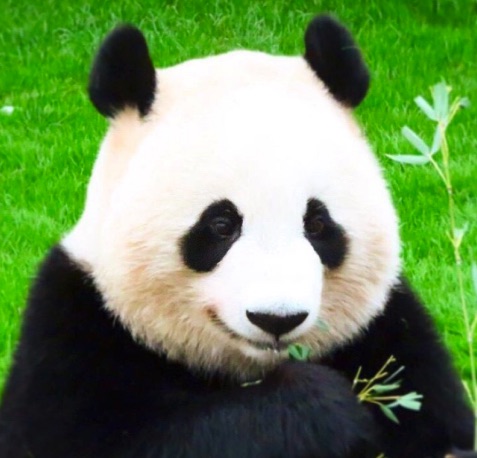
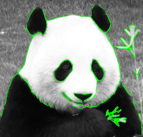
Just for fun, I also tried my edge detector on this image 🙂